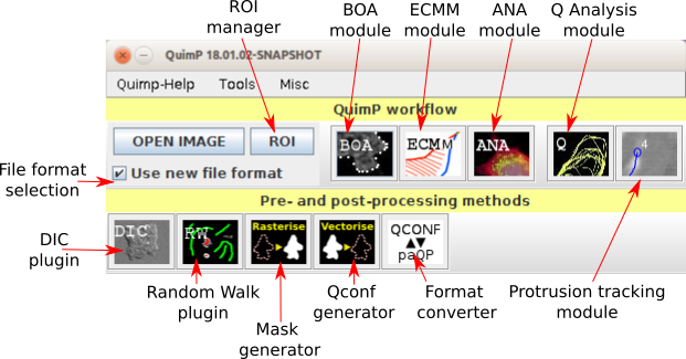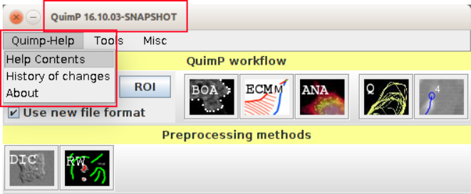
Figure 1: The QuimP bar
Version: 19.04.03-SNAPSHOT
Web site: http://www.warwick.ac.uk/quimp
This manual is available on GitHub. Feel free to fork it and make pull requests!
https://github.com/CellDynamics/QuimP-_Doc
Manual compiled on Friday 26th April, 2019 at 07:39
The full text of QuimP license is available at https://pilip.lnx.warwick.ac.uk/LICENSE.txt.
Please, make the following citation in any publication related to our software:
”QuimP [1] used in this study was developed at the University of Warwick with support
from BBSRC (BBR grant BB/M01150X/1).
[1] Piotr Baniukiewicz, Sharon Collier, Till Bretschneider QuimP: analyzing
transmembrane signalling in highly deformable cells. Bioinformatics, Volume 34, Issue 15,
1 August 2018, Pages 2695-2697, doi: 10.1093/bioinformatics/bty169
The user manual exists in two versions, final and development. The final documentation is (usually) related to the current official release of QuimP, whereas the development version evolves together with the software, following upcoming features, bugfixes, etc.
The most recent documentation can be downloaded from:
The key features of releases:
A changelog can be found at the QuimP web page at: https://pilip.lnx.warwick.ac.uk/site/changes-_report.html. Version of QuimP you are running as well as the version history can be viewed directly from the QuimP Bar plugin (subsection 1).
If you find a bug or have specific feature requests, please contact the QuimP developer:
p.baniukiewicz@warwick.ac.uk
Consult our Wiki page for installation details:
http://warwick.ac.uk/quimp/wiki-_pages/
Matlab routines and walkthrough data mentioned in this section are available from QuimP web page2 .
Check also our latest publication: Piotr Baniukiewicz, Sharon Collier, Till Bretschneider; QuimP Analyzing transmembrane signalling in highly deformable cells, Bioinformatics, which contains many examples and workflows in supplementary materials.
Simple example of processing QuimP datafiles in Python is available at our GitHub account3
The folder QuimP_walkthrough_files contains 3 tiff image sequences which you can analyse (images are courtesy of Evgeny Zatulovskiy, Rob Kay Group, MRC Laboratory of Molecular Biology).
You can find the results from above analysis in example_output folder, exemplary post-processing in Matlab are available for viewing here4 .
Step 1. Open ImageJ and launch the QuimP bar [Plugins → QuimP → QuimPBar]. Open the image QW_channel_2_seg.tif. Launch BOA from the QuimP bar.
Step 2. At the prompt check the scale is correct (2 second frame interval, pixel width 0.2 microns).
Step 3. Using the polygon selection tool, create a selection encompassing the cell. This can be very rough. Click Add cell.
Step 4. Adjust the parameters to get a good segmentation. Click SEGMENT and wait for completion. You can also restore experiment configuration from QW_channel_2_seg.QCONF file from example_output folder.
Step 5. Scroll through the sequence to check the segmentation result using either the scroll bar or mouse wheel. The segmentation should have completed to the last frame. If not, we will truncate the segmentation. Scroll to the last frame which successfully segmented and click Truncate Seg. Click FINISH, and provide a name for the analysis (e.g. ‘QTest’).
Step 6. Launch the ECMM plugin from the QuimP bar. It does not require an image. When prompted, locate the QuimP parameter file you just created (e.g QTest.paQP). ECMM will run. You can view the result and close the image.
Step 7. Open the image QW_channel_1_actin.tif. With it in focus, launch the ANA plugin, and again select your parameter file. Choose a sensible cortex width (e.g. 1.5 microns). Make sure ‘save in channel’ is set to 1, and normalise to interior is ticked. Click ok. When complete, ANA will show the sample locations for the last frame.
Step 8. Close QW_channel_1_actin.tif, and open QW_channel_2_neg.tif. We will record another channel for good measure. Repeat the last step, but with the channel 2 image, this time storing data in channel 2 (which is the default), and tick Sample at Ch1 locations. ANA will now use the same sample points as computed for channel 1 (useful if you want to compute ratios between channels).
Step 9. Launch the Q Analysis plugin, and again choose your parameter file. Check your scale is what you expect at the top of the parameter window. We will use all the current defaults, so click RUN. Inspect your maps, all of which are automatically saved to disk.
Step 10. The displayed images have been scaled to cover the colour space. The raw values have been saved as text file, with the extension .maQP (e.g. QTest_0_fluoCh1.maQP). You can view them in ImageJ by opening them via [File- > Import- > TextImage...]. Note that latest versions of QuimP store these files inside QCONF configuration file. One can retrieve them by using Format Converter (see section 14).
Step 11 We will now switch to MATLAB to plot some of this data. Open Matlab and open the script file walkthrough.m, which will guide you through loading and plotting data. You can use the output provided in the QuimP package, called QWalkthrough, rather than your own.
In this example you will perform analysis similar to subsection 6.1 but with help of ImageJ macro. Note that this approach requires already segmented image provided as binary or grayscale mask (we use Segmentation.tif from walkthrough files). More about converting masks to QuimP format is given in subsection 8.5. Below you can find exemplary macro that performs the same anaysis like that described in subsection 6.1
For latest and actual version of macro check walkthrough data archive 5.
There are four stages which are usually performed when tracking cells using QuimP, each handled by a different plugin (section 2).
Additionally, there are data pre-processing plugins available such as:
A plugin can be launched from either the [Plugins → QuimP] menu, or from the QuimP bar (opened via [Plugins → QuimP → QuimPBar]). Running a plugin will either require an image and/or a QuimP parameter file (with extension .paQP or .QCONF) generated by BOA (see section 14 for details). Demanded file format can be pre-selected by File Format Selection tick box. This selection influences all QuimP modules, even if started directly from Fiji plugin menu. Plugins must be executed left to right, although steps can be repeated without re-running previous plugins and fluorescence measurements performed by ANA can be skipped entirely.
Once complete, data can be analysed in Excel or MATLAB.
QuimP allows for simple integration with Omero database. Currently supported is uploading and downloading QCONF experiment files to and from Omero. In both cases QCONF file and related image are loaded or saved to disk. For more detail consult short help available in OmeroClient module (Tools → Omero client).
QuimP utilises an active contour method to segment cells from the background of an image. Typically, this
will be a time lapse movie containing a fluorescence channel, captured from a confocal microscope,
but the BOA plugin will segment any image which has bright objects on a dark background
(note that phase contrast images can not be segmented with this method). Attaining the best
image for segmentation may require some pre-processing, such as the combining of available
fluorescence channels (the ideal case is that of an evenly white cell on a black background).
section 3 describes the active contour method and provides insight as to BOA’s parameters.
It is expected that objects being segmented have intensity higher than background. Active contour
method implemented in BOA will not work for other cases.
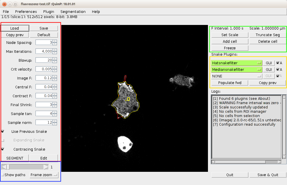
The BOA window is presented in section 4. There are four highlighted areas, which contain tools and allow to adjust settings for segmenting and displaying images, and postprocessing of segmented contours.
Step 1: Open an image and ensure the correct scale. QuimP can segment from a single image, or from an image stack (but not from a hyperstack). Only 8-bit images can be used for segmentation and so you will be prompted to convert to 8-bit if required. QuimP uses the scale properties of the image to scale all output to microns (pixel size) and seconds (frame interval). ENSURE YOUR SCALES ARE CORRECT within [Image → Properties...]. On launching, BOA will prompt to check your image scale. The scale is recorded by BOA and stored in the parameter file for use in the rest of the analysis.
Step 2: Launch the BOA plugin
Unlike previous versions, BOA no longer requires selection of cells prior to launching, but you can do so. Launch BOA from the QuimP bar or menu. The BOA window is now a fully functional ImageJ window that allows the user to perform any ImageJ function, such as drawing, creating ROI’s, or zooming while the BOA plugin is in use. section 4 shows the BOA window. The image scale is displayed at the top right. To adjust the scale click Set Scale.
BOA can segment one, or more cells, each beginning and ending at any frame you wish. In addition, you can manually edit any segmentation at any frame, add/delete cells, truncate segmentations, and adjust the segmentation parameters for individual frames.
Step 3: Adding and deleting cells.
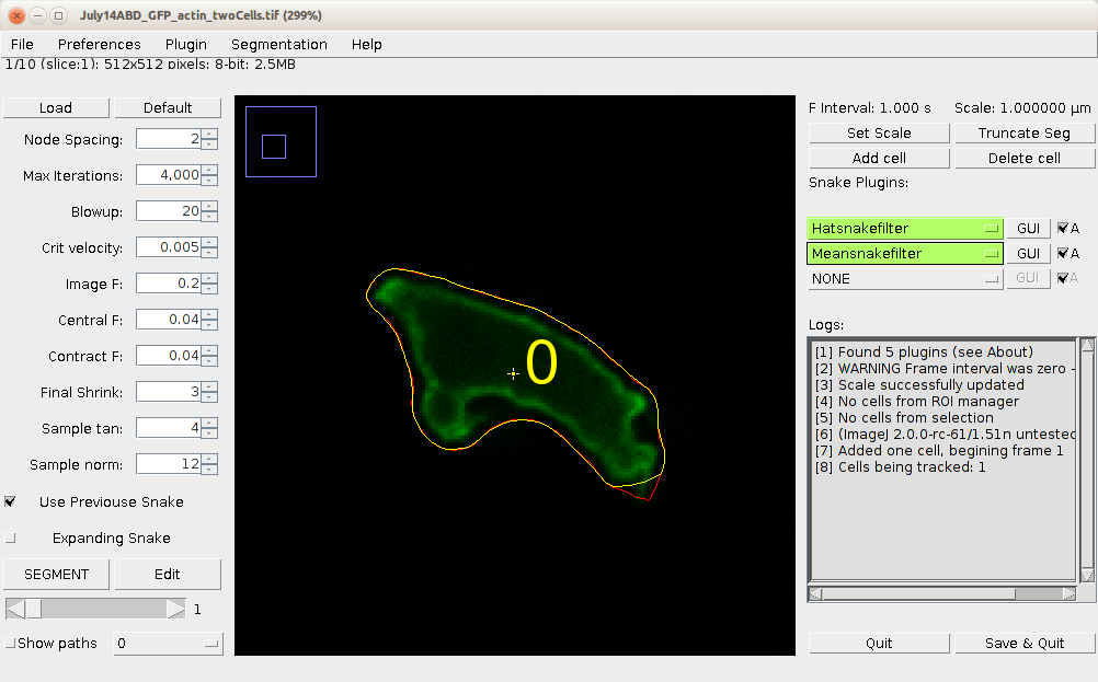
To add a cell first scroll to the frame that you want to begin the segmentation at (either with the mouse wheel, or slider). Using either the circular, rectangular or polygon selection tool, draw an ROI (region of interest) around a cell, and click Add cell. BOA will immediately attempt to segment the cell at the current frame. If convergence is successful, the result is displayed as an image overlay. The cell is also given an identification number. If the segmentation fails for some reason, the parameters can be adjusted (see below). You do not need to re-add the cell.
Additional cells can be added in the same way. The active contours surrounding each cell will interact with one another and prevent contours crossing over to other cells. This capability is particularly useful in situations where cells come into close contact, which often disrupts the segmentation process.
If you are not able to find optimal parameters for many cells at once, you can select only one cell then follow points below and at the end use Freeze button to block further modification of this cell. Then repeat the whole process for another cell. Note that Freeze freezes the whole sequence and one can has many sequences frozen at one time.
To delete a cell click Delete cell, and then click the centre marker of a cell, on any frame where a segmentation is visible. Hit the same button again to leave delete mode.
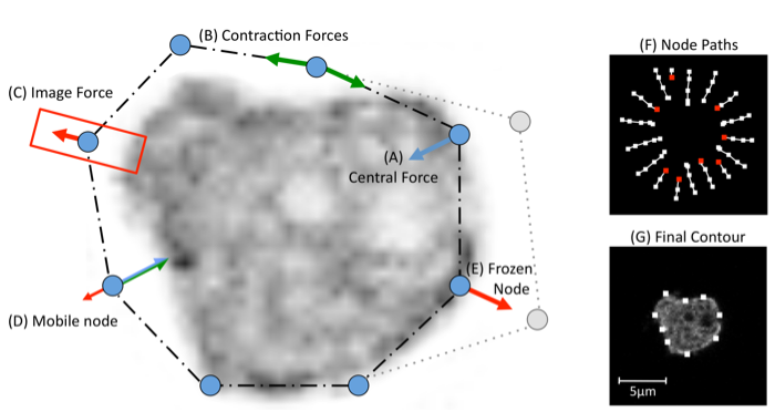
Step 4: Adjusting segmentation parameters.. When a parameter is altered, BOA immediately re-computes the segmentation for all cells on the current frame with the new parameters (all cells share the same parameters). Each has a minimum/maximum value that can not be exceeded. To alter a parameter either enter a value into the text box, or use the arrows to increase/decrease in steps. The key to attaining a good segmentation is the balancing of the 3 forces. First, try adjusting the Image F parameter to improve the result. Parameters can be set for each frame separately. One can also freeze cell to exclude it from further processing.
The parameters are as follows:
Buttons and checkboxes:
Previous segmentation for your image can be loaded back into BOA by hitting load and selecting a QuimP parameter file with the file extension either .paQP or .QCONF. Parameter values alone can be loaded by declining to load associated snakes. Button Default sets above parameters to their default values and recompute current frame. The Copy prev button will copy segmentation parameters from previous frame to the current one and re-run segmentation.
Enabling the tick box labelled Show paths will display a trace of the snake as it contracts. Nodes colour pixels white as they move towards the cell boundary. This view can be useful for diagnosing why a segmentation fails.
Step 5: Segmenting multiple frames. When happy with the segmentation on the first frame, hit SEGMENT to segment the cell (or cells) in the following frames. Segmentation parameters from starting frame will be copied to subsequent frames. Any outlines already existing on these frames will be overwritten. The algorithm may fail at a particular frame and a warning will be printed to the log window, at which point you can alter parameters.plugins. This process can be stopped in any time hitting SEGMENT once more.
Step 6: Correcting segmentations. In the case of failure, or incorrect results, you have 3 options:
You can use also Zoom freezes feature from Preferences to change Frame Zoom behaviour. If Zoom freezes is ticked on, Frame Zoom freezes all already segmented cells except that currently zoomed. Then any modification will apply only to magnified cell.
Step 7: Save the results. Click Save and Quit. The saved cell outlines are those visible on the yellow overlay. For new QCONF format selected (default) only one composite file is outputted. Otherwise a set of files will be saved for each segmented cell (see section 14 for description differences between new and old data file format). A cell’s ID number is automatically added to filenames.
Enter a name for the analysis (file name extensions are added automatically). BOA outputs files with a QCONF extension for new fileformat or .xxQP for old one7 .
Files extended with .paQP contain file paths and parameters associated with a particular analysis. When running other QuimP plugins, it is the .paQP file which you must select to continue an analysis (see subsection 14.2).
Files extended .snQP contain all data associated with individual nodes of an outline, including pixel coordinates, local cortex intensity, local membrane velocities, and tracking data (see subsection 14.3).
Files extended .stQP.csv contain average statistics per frame, and can be opened directly in Excel as a ‘comma separated file’ (see subsection 14.4).
The BOA plugin alone outputs many useful statistics regarding cell morphology and migration, without the need to run any further analysis. Simply open the .stQP.csv file in Excel, or use the accompanying scripts to load data into MATLAB (see section section 16).
BOA module supports external plugins for post-processing outlines on current frame. Plugins are standalone jar files that can be developed by other scientists and distributed independently from QuimP. Available plugins are discovered when BOA launches by scanning default location, which is Fiji/plugins folder. There is no need of any additional action, discovered plugins are available in filter stack on right (see section 4). There are three slots in the stack. Filters are applied in order from most top to bottom, next filter starts with contours returned from the previous one. Any action on filters relates only to current frame (thus each frame can have different filter stack) unless SEGMENTATION button is clicked. Automatic segmentation propagates most recent configuration (that means all options available in BOA window) from starting frame to all subsequent frames. Modified contour is drawn in standard yellow colour, whereas red denotes original unprocessed result of segmentation (subsection 5). Any further processing in QuimP workflow (e.g. ECMM or ANA) applies to filtered outline. Refer to subsection 8.1 for other options related to filters. Frozen cells (section 8) are also excluded from processing by filters.
If filter contains an user interface, it can be accessed by GUI button (subsection 5).
Default installation of QuimP contains four BOA filters:
Filters that have been discovered and properly loaded are marked in green colour. This is standard behaviour when user start analysis from scratch. If BOA configuration has been restored from QCONF file, filters (if any was used) are displayed in red colour to denote that result of segmentation (that is stored in QCONF file together with raw unprocessed outlines) was processed by filter stack but none of those filters is loaded yet to BOA. In this mode user can browse through frames, check segmentation parameters, etc. even if a filter is physically not available in his configuration. Option Plugin→Re-apply all will try to load all necessary filters from disk and apply them to each frame where they were used. Note that this operation will recompute all outlines on frames where filters were used and replace loaded results with those evaluated.
If you run into difficulties attaining a good segmentation, there are a few tricks that may help. If the width of your cell is around 20 pixels or less try artificially increasing the size of the image with some form of pixel interpolation selected ([Image → Adjust → Size]). This should aid sampling of the image and allow nodes to enter concavities with greater ease (note, all subsequent analysis must be performed on the image at the new resolution).
If your images are particular noisy, and cell’s appear very grainy, you may try applying a weak Gaussian blur to smooth them ([Process → Filters → GaussianBlur]). This should make for more reliable sampling of the cell’s interior.
Remember to recalculate the scale of the image when resizing, and to perform intensity analysis on the rescaled image without any interpolation.
Another common approach to improving image quality is to remove background noise using a ‘blank’ image, one taken without any cells in the field. This is particularly useful for removing shadows of dirt on the optical equipment, and correcting uneven backgrounds.
The QuimP supports creation of Snake outlines directly from binary masks. As the active contour method is not used in this case, one can use another segmentation algorithms (e.g. Random Walker method) to deal with problems that typically occur for active contour such as e.g. bad segmentation of cavities.
To use binary segmentation, either black-white mask (8-bit image in ImageJ) or grayscale images should be obtained in any other way, e.g. by using alternative segmentation tools. It has to be size of segmented image that is already loaded to BOA plugin. The number of slices in mask file should be less or equal to the number of slices present in segmented image. The background pixels must have value 0 whereas objects can be defined by any other values within the range 1-255. This plugin is capable to perform simple cell tracking between adjacent frames. If input mask is binary then cells are assigned to the same track by testing their overlapping between frames. For grayscale images, numeric values of pixel intensities are used.
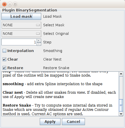
The binary segmentation plugin can be launched from BOA menu (Segmentation → Binary segmentation) or as standalone module from QuimP Toolbar. The latter method supports also IJ macros. If one calls this plugin as separate external module from QuimP Toolbar or IJ menu, it will produce Qconf file in the same way as BOA module does. This file can be than passed to other QuimP modules for further analysis.
The mask can be either loaded from separate file (ImageJ formats are supported) or selected among already opened images in ImageJ. Results of segmentation are displayed in real-time on BOA window immediately after clicking Apply. Cancel closes the plugin window leaving last results of segmentation in BOA. If Clear is selected each use of Apply will clear current outlines in BOA. If it is unselected, outline will be added to BOA. Note that each click on Apply will create new outline even if non of plugin parameters is modified. Resulting outline can be smoothed by e.g. MeanSnakefilter available in the plugin area (see section 4). Filter can be applied for selected frames only or populated for the whole sequence by (Plugin → Populate plugins)
To extract data on local membrane velocity QuimP utilises our Electrostatic Contour Migration Method (ECMM). Nodes that form a cell outline at time t are mapped onto the segmented outline at time t+1. The distance a node migrates during the mapping process, and the frame interval, determines the local membrane velocity at the node’s position. If you only have a single frame there is no need to run this plugin. ECMM edits and adds to data already contained within an .snQP file.
Step 1: Launch the ECMM Mapping plugin, and open the desired .paQP file when prompted. There are no parameters that require manual setting.
Step 2: Inspect the results. The blue outline represents the cell outline at time t, the green at time t + 1. Green circles, overlaid with crosses, denote intersection points that have been validated and used for calculating sectors. Red lines denote paths taken by migrated nodes. Nodes that fail to map correctly are highlighted in yellow. Failed node (FN) warnings are displayed along with a running total (in brackets) of the number of failed nodes in the whole sequence. The log window will display progress and warnings.
If a node fails to map it is simply ignored, the effect of this is a small reduction in mapping resolution at the nodes location. If the process fails to map the majority of the nodes correctly, then a new segmentation will have to be performed (try using a different node resolution or changing the image resolution).
The details as to the workings of ECMM can be found in our publication [3]. The current implementation includes several significant improvements. It is not necessary to understand the method, only the format of the tracking.
At frame t = 1 a node is randomly chosen as being node zero, n0. Other nodes are then assigned a position according to their distance from n0 along the cell perimeter. The length of the cell perimeter is normalised to 1, hence the position of a node which is exactly half way around the perimeter will be 0.5 (see subsection 7a).
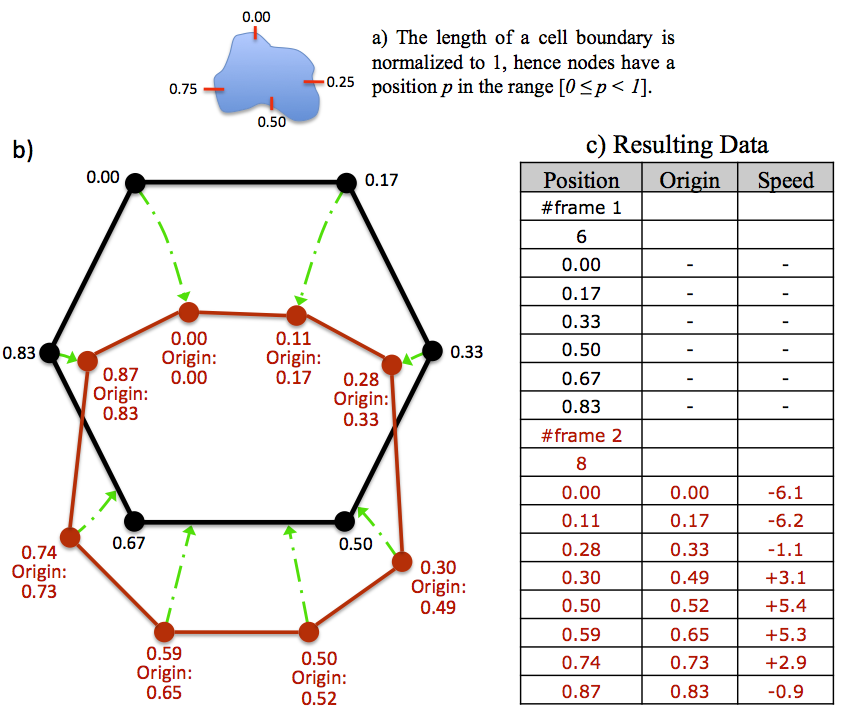
The nodes of the outline at t = 2 also have positions assigned, but in addition have an origin. This represents where a node originated from on the t = 1 outline. For example, a node with an origin of 0.5 originated from position 0.5, exactly half way around the outline at t = 1.
It should be realised that this method of tracking is sub-node resolution. By simply interpolating the positions and origins of nodes, any real number position on an outline can be tracked at sub-node resolution, for as many frames as desired. See subsection 14.3 for the format of data output, and subsection 16.3 for using ECMM data within MATLAB.
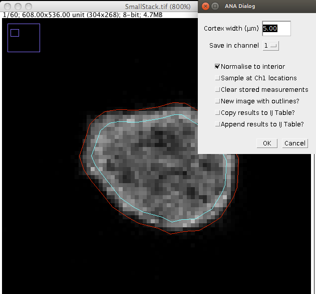
QuimP samples the intensity of pixels from within the cortical region of a cell. At each frame, nodes of the cell outline are shrunk inwards to form an inner outline. The amount of shrinkage is specified by the user, and relates to the estimated cortex width. Nodes are migrated inwards towards the inner outline, while simultaneously measuring pixel intensities (a 3x3 average). A nodes fluorescence intensity is the maximum recorded as it migrates across the cortex. ANA can record data for up to 3 separate fluorescence channels.
Step 1: Open an image stack containing the desired fluorescence channel. This may be the same stack used for cell segmentation, or one containing data from another channel. Ensure the opened stack has the same resolution and number of frames as that used for segmentation.
Step 2: Launch the ANA plugin and open the desired .paQP or (recommended) QCONF file when prompted.
Step 3: Enter a value for the cortex width (μm) and choose a channel. The inner and outer outlines are displayed on the image. Changing the cortex width will update the image overlay. Choose a channel to record data in from the drop down menu.
ANA provides 5 further options
Click OK.
Fluorescence data associated with specific nodes is saved in the QCONF file and additionally in .stQP.csv.
Step 4: For further channels, open the next channel image and re-run ANA.
Data within QCONF file (or .snQP and .stQP for old path10 ) files can be read into Matlab at this point, but motility maps have not yet been generated11 . The Q Analysis plugin will build spatial-temporal maps of motility, fluorescence, and convexity, and also several other maps to aid analysis. In addition, vector graphics are produced using the Scalable Vector Graphics format. These include a cell track in which all cell outlines are overlaid and coloured according to frame number, and a motility movie in which nodes are coloured with a user specified data type.
Step 1: Launch the Q Analysis plugin and open the desired .paQP file when prompted.
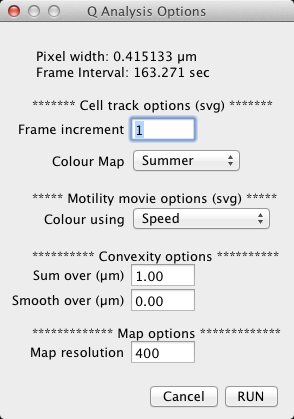
Step 2: Enter parameters to the options dialog. The parameters are as follows:
The images produced are for visualisation only, as they have been scaled to fill the RGB colour spectrum. Vertical image scale is set to frames (frame zero at the top), horizontal to the normalised length of the cell perimeter (0,1]. Import .maQP files as text images for further analysis in ImageJ. See Section subsection 14.5 for details and analysis of maps.
Differential interference contrast microscopy (DIC) enhances the contrast in unstained, transparent samples. DIC images can be easily interpreted and analyzed by biologists due to high resolution available and excellent contrast generated by steep gradients in optical path lengths and phase shifts between the two polarized beams. Nevertheless, very characteristic bas-relief observed in DIC images is the source of problems in automatic analysis of these images. The image contrast and the same the objects boundaries are well defined in the shear angle but in direction perpendicular to it there is no contrast against to background and thus a lack of distinct edges of object. Moreover, strong gradient of image intensity at shear angle negatively influence standard image processing methods like global thresholding or edge detection producing insufficient results, with discontinuous regions or edges.
The DIC plugin provided with QuimP allows to convert DIC samples into form more suitable for segmentation and further image processing. The local contract for any cell in reconstructed image is well defined in every direction and the intensities of pixels take only positive values (in relation to a mean intensity level). The algorithm implemented in QuimP is described in [2]. Either single images or time lapse movies from DIC microscopy can be processed.
Step 1: Open an image. Once loaded into ImageJ/Fiji click DIC filter in QuimP bar. Only 8-bits images are supported (256 gray levels).
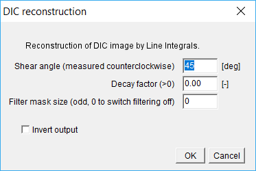
Step 2: Set correct parameters There are two important parameters: Shear angle and Decay (Fig. subsection 10). The Shear parameter is the shear angle of DIC microscopy measured counterclockwise, whereas Decay is described in details at [2]. The Decay factor depends mainly on the size of cells and the best results are usually achieved experimentally. Invert output option inverses colorscale in reconstructed image.
Reconstructed image can be affected by linear pattern that can be filtered by running mean filter activated if Filter mask size is greater than 0. Smoothing filter is applied before processing for angle perpendicular to given Shear12 .
If objects (cells) in reconstructed image are darker than background, the image should be inverted before further processing in BOA module. One can use ImageJ option Edit→Invert or tick Invert output in plugin window. Refer to section 8.
The Random Walks Segmentation algorithm is described in the paper [1]. It belongs to the class of supervised segmentation algorithms what means that the user interaction is needed. In RW method a user has to specify a small set of pixels belonging to the desired object and (possibly) a set of pixels belonging to the background. Those pixels are called seed pixels and in this plugin they form the seed image. The seed image must be the size of segmented image whereas, the number of layers can be either equal to number of layers in segmented image or set to 1.
This plugin supports also multi-object segmentation, where user defines several foreground objects (up to 255). For this case, the output is a grayscale image where each unique object is marked by different colour, starting from 1.
Segmentation is run in two sweeps. First one gives rough segmentation whereas the second one produces final result. Second sweep uses binary mask produced by the first step as an input after filtering it by selected Binary filter. Second sweep can be disabled by setting Gamma 1 to 0 (disabled by default, use with care as it can give unpredictable results in some cases). By default second sweep uses half of defined iteration number.
For best results, the background seeds should be drawn close to foreground objects.
Implemented algorithm uses iterative scheme with three possible stopping criteria:
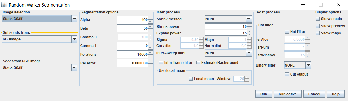
The RW plugin can be called outside of QuimP from the QuimP Bar, from IJ macro or directly from API. The main interface is presented in subsection 11. The window is divided into eight sections:
Image section - here user can select image that will be segmented. It must be grayscale image either 8 or 16 bits.
Seeds section - defines source of the seed image. The following options are available:
Dynamic section - its content depends on selected seed source.
Segmentation options - controls segmentation process. Options available here:
Inter-processing section - it controls how binary masks should be transformed to seeds internally. This process applies when seeds are given as resultSeeds sections of segmentation from other method (Mask image or QCONF file) or there is only one slice of seeds provided (RGB image). Binary mask is shrunk by algorithm selected in Shrink method with Shrink power. Results define object’s seeds for next frame. Then, the same mask (unmodified) is expanded by the same algorithm but with Expand power and then inverted to define background seeds for the next frame. Options available here are:
Generally, non-linear shrinking try to maintain shape of original contour but constricting it more around concave regions of the outline, that should reduce accidental miss-labeling the background.
Local mean - this option can improve behavior of the algorithm in areas with high gradient of intensity, usually at cell cortex, preserving cell boundaries. This method works only with seeds provided as Mask image or QCONF file. Moreover, masks should be larger than the object itself. Window parameter stands for the size (odd) of the sampling window used for computing local mean intensity.
Post-processing section - it covers filtering of results applied after segmentation. The options are:
Display options section - allows to show real time preview of each segmented frame and seeds computed as results of Iter-processing binary masks. This option can be used for verifying Shrink power and Expand power settings. Show maps display raw unscalled probability maps for each seed. This option does not work with stacks, only probability maps for last segmented frame are displayed.
ROI collector is available after selecting ROIs in Seeds section. This tool uses ImageJ ROI Manager to store ROIs that denote foreground and background seeds. The ROIs need to obey certain naming criterion, such as [LB][Id]_[No], where LB can be either fg or bg denoting foreground or background seed respectively, Id is unique number of foreground object (only one or none background seeds are allowed) and No is a sequence number of ROI for object of specified Id (a seed for one object can be specified by several separate ROIs).
The ROI collector tool (subsubsection 13) manages proper naming of ROIs in the ROI Manager. After launching, the ROI Manager will be opened and its content erased.
User can label an image using standard ImageJ ROI objects and then click New FG or new BG to add current selection to ROI Manager. Each next use of New FG will add new foreground object. If certain object ought to be labeled by separated ROIs, they should be added to ROI manager first (by Add button) and then New FG should be clicked. All ROIS in ROI Manager that do not follow specified naming convention are renamed and assigned to one object by New * buttons. To finish labeling and transfer ROIs to the plugin click Finish button.
If segmentation ends too early (e.g. result is very similar to seeds) one can open Fiji Console (Window→Console) and check reason of stopping and relative error. If process stops due to reaching relative error in the first few iterations, one can adjust Rel error accordingly.
This plugin can convert cells contours into binary image mask. The cell shape is represented by white area being a filled cell contour whereas the background in black. Masks are widely used in computer graphics for selecting regions of image for processing and analysing. ImageJ is also equipped with relevant procedures that allow for explicit processing masked regions. Therefore, this plugin make it possible to continue analysis of the sample outside the QuimP infrastructure.
Mask Generator plugin works with QCONF files saved by BOA module. It is not possible to use it with old file format (paQP) unless it has been converted to QCONF by Format Converter (available from QuimP Toolbar menu). By default, the mask image is displayed on the screen and saved on disk at location of input QCONF file with suffix snakemask.
This plugin supports ImageJ macro language. Use Macro Recorder to discover the syntax.
Protrusion Analysis module allows investigating protrusion formation and dynamics. The module requires QCONF file that contains full description of QuimP analysis. Particularly, the BOA, ECMM an Q Analysis modules should be run on QCONF before using Protrusion Analysis.
Arbitrary points of interest can be selected directly on the cell contour or imported from ROI Manager.
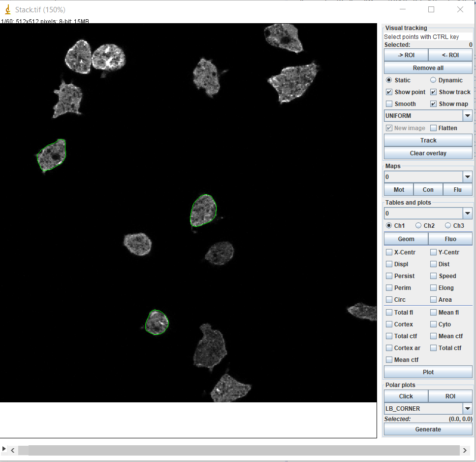
The user interface is shown below.
There are four sections on the left side of the user interface:
The contours of the cell consist of vertices, internally each vertex v for cell c is represented by two coordinates: position along outline and time (frame), v =< p; t >. The same coordinate system is used for maps generated by Q-Analysis (Maps section of the UI). The vertical axis represents time, with frame 1 at the top. The horizontal axis represents positions along the cell outline, the length of which has been normalised to 1 at every frame (see subsection 14.5). Resolution of horizontal axis can be configured in Q-Analysis module (default value is 400). Resolution of vertical axis equals number of frames in the sequence. These both values are stored in the QCONF file.
If points selected on the cell contour in the main view of the plugin are exported to ROI manager, they are converted to screen coordinates using configured resolution for positions along the cell outline and number of frames in the sequence (e.g. for default resolution of 400 and 100 frames, point selected at frame 50 in the middle of the contour will have coordinates x = 200, y = 50). Additionally cell number is encoded in the ROI name as suffix cell_N_X, where N is the cell number and X stands for point number.
Reverse operation - importing points from ROI expects the same naming convention unless the user will press and hold CTRL key to import all points to the outline of the cell 0. ROI coordinates also should follow guidances given above, they will be converted to ¡position;frame¿ on the outline. Position is selected as the closest vertex on the outline to the input point. Not that ROI can be also shapes, which allows to select more than one point at once.
Tracks are generated from selected points on the cell outline. Selections can be made directly on the outline or imported as ROIs.
In this scenario we are interested in detecting protrusions and tracking them. We use motility map to find out points with highest velocity and then we will track them in the plugin.
The latest QuimP introduces a new file format called QCONF13 . The QCONF is based on human-readable JSON format and it is designed to hold all results evaluated by QuimP on every stage of data processing, together with configuration parameters, algorithm settings, etc. (check subsubsection 14.1.2 for details on QCONF structure). Initially, the QCONF is generated by BOA plugin together with stQP file (the same statistical measurements are also contained in QCONF, stQP file is saved separately for convenience sake). Remaining modules depend on QCONF, thus they read and write all data from/to this file. The QCONF is not replacement for ”old” formats - it rather extends them and allows for easy sharing of results between different QuimP modules, restoring work from last point and keeping the whole QuimP configuration in one place.
Currently, QuimP understands both formats, but its behavior depends on the status of tick box available in QuimP Toolbar (section 2) and on format loaded to module:
Relations between module and file are summarized in subsection 1. Legend for subsection 1 is as follows:
Note
The QCONF file can be loaded to Matlab using one of the free JSON parsers (tested with
JSONlab16 ).
| paQP | snQP | maQP | stQP.csv | QCONF | pgQP | svg | tiff | |
| BOA | N | N | N | N | N | |||
| ECMM | C | M | ||||||
| ANA | M | M | M | M | ||||
| Q Analysis | N | M | N | N |
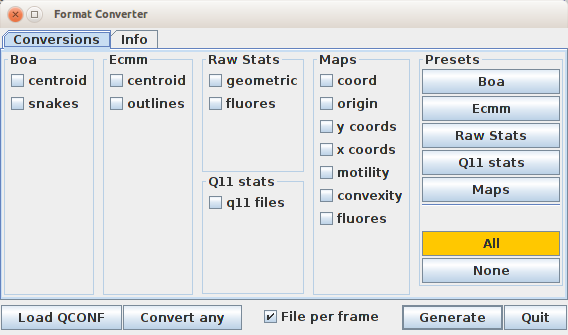
QuimP supports conversion between old paQP and new QCONF formats. Simple tool for this purpose is available from the QuimP bar (see section 2) under Tools menu or in extended version as separate module (see subsubsection 15). The module additionally allows to extract numeric data from QCONF and save them in user friendly csv format.
Conversion between formats - Convert any button
Conversion tool is available from either the QuimP bar or Format Converter module under Convert any button. After selecting proper input file - QCONF or paQP, the opposite format is saved in the same folder. The following rules will apply:
Extracting data from QCONF format - Load QCONF button
Format converter module (subsubsection 15) allows to save selected parameters evaluated during QuimP workflow and stored in QCONF file as separate csv files. Some parameters (like e.g. those under Raw Stats) coincide with content of snQP or stQP.csv files. Data extraction is applicable only to QCONF files that should be loaded by Load QCONF button. Conversion process is initiated by Generate button. Output files are saved in the same folder as input QCONF.
Simple example of processing QuimP data files in Python is available at our GitHub account17 .Notebook contains also scheme of QCONF structure generated by tool available in the same repository.
Similar approach can be used in any language supporting reading JSON files. One can also convert QCONF to old file format, based mostly on widely understood csv files, and follow e.g. this example in Matlab18
A parameter file contains text and has the extension .paQP. Both QuimP’s plugins and Matlab functions use the parameter file to locate files associated with an analysis and also to store data such as the pixel size, frame interval, and start frame. In addition, it stores the parameters used for segmentation (the last used parameters).
The first line identifies the file as a QuimP parameter file, and contains the creation date. The second is random identifier. The third is the absolute path to the image used for segmentation.
In general, the contents of a parameter file should not be changed, but you may wish to alter the paths to image files if you later move them.
The .snQP file contains data relating to the nodes of cell outlines (snake is a reference to active contours being described as snakes). Comment lines begin with a #. Data for frame f begins with the comment line #frame f, followed by a single integer value indicating the number of nodes that make up the outline (N). The following N rows hold the data for the nodes. The columns are as follows:
It is possible to store data for 3 fluorescence channels ($ = {1, 2, 3}) within the .snQP file. Missing data is denoted by negative values.
The statistics file, with the extension .stQP, contains whole cell statistics for each frame (rather than node associated data). Data is written as comma separated values which can be opened easily as a spreadsheet. The file is split into two section. Data in the top section is computed by BOA and relates to cell morphology and movement of the cell centroid. Data in the lower section relates to cell fluorescence and was computed by ANA (data is listed separately for all 3 available channels). Missing data is denoted by -1.
The cell centroid is computed as the weighted centre of the polygon formed by the cell outline. The measures computed by BOA are as follows:
This file is generated and updated regardless of selected file format (QCONF or paQP). Refer to subsection 1
 . A value of
1 reveals the cell’s outline to be perfectly circular.
. A value of
1 reveals the cell’s outline to be perfectly circular.
The measures computed by ANA are as follows:
The images produced by Q Analysis are spatial-temporal maps of motility, convexity, and fluorescence. The vertical axis represents time, with frame 1 at the top. The horizontal axis represents positions along the cell outline, the length of which has been normalised to 1 at every frame. Outlines can be thought of as having been ‘cut’ at position zero, laid along the horizontal axis, and stacked below one another, hence maps are cylindrical (wrap around onto themselves on the horizontal axis).
The node randomly designated as begin node zero (n0), at frame 1, is mapped to the top left pixel. Data from ECMM is used to track the position of n0 throughout all the frames, and is always positioned at the left most pixel at each frame. All other nodes are positioned along the horizontal axis according to their distance from n0 along the cell perimeter. Values between nodes are estimated using linear interpolation.
If the number of frames is below the specified map resolution, then maps are scaled vertically, hence a row of pixels may be an interpolated value between frames.
As well as producing .tif images, maps are also saved as text images with the extension .maPQ. Unlike the .tif maps, these are not scaled vertically, so each line of values contains the data for a single frame. It is these maps that should be used for further analysis.
Similarly, four additional maps are produced to aid further analysis:
Files extended with .svg can be viewed natively in most internet browsers (Windows Explorer requires the Adobe SVG viewer), or opened and edited in graphics software ( e.g. Inkscape, free software for mac). The Scalable Vector Graphics (svg) file format can be viewed at any desired resolution.
This file stores configuration of plugin stack together with configurations of active plugins (see section 4 and subsection 8.3). This file is not related to any loaded data therefore it can be exchanged between projects. Complex plugin stack configuration is stored also in QCONF file.
Most of QuimP modules support ImageJ macro language but syntax of the command (especially parameters passed to the module) differs from that commonly used by other ImageJ plugins. Use Macro Recorder tool to discover parameters supported by plugin. Note that any file name or path should be enclosed in parentheses if it contains spaces. Windows users should use slash symbol in path names (e.g. c:/Users/myfile.QCONF). Quote character is not allowed in parameter string. Skipped parameters get their default values, therefore output from Macro Recorder can be greatly reduced by removing options that are not used or unchanged.
Note that macro strings are outputed to Macro Recorder only if plugin is run from Menu. It does not work if plugin has been started from QuimP Toolbar.
Archive with Matlab routines mentioned in this section is available on QuimP web page (section Download QuimP)19
Matlab routines work with old data format only (*.paQP, *.snQP, etc.). To use them with QCONF file, it has to be first converted to the old format by Format Converter (section 14). It is also possible to load QCONF to Matlab using JSon readers.
QuimP outputs a large amount of data for each cell analysed. You may want to write custom scripts for analysis, but we provide a set of MATLAB functions to remove the hassle of loading/organising data, and performing simple operations, such as plotting maps. We hope to make data as accessible and as explorable as possible to allow adaptation to a users specific goals.
Help documentation is included with each function which can be accessed in the usual way by typing help functionName at the MATLAB command prompt. At the end of this document is a walkthrough analysis using the provided test images (see subsection 6.1).
The first step is to launch the script readQanalysis.m which handles loading of data from multiple cells. Given a directory, it will search that directory, and all sub-directories, for .paQP files. For each parameter file that is found an analysis structure is built. As data is read from sub-directories, you may organise your separate analyses into sub-directories, but placing all files into the same directory is still possible. Missing files are skipped, hence it is not necessary to have run all the QuimP plugins.
Loading data relies on the maintenance of file names imposed by the QuimP plugins, and requires associated files to be present in the same directory as the parameter file. The exceptions to this are the images used for segmentation and fluorescence measurements. Paths to these images are stored in full to allow separation of analysis files from image data. If images are moved, and subsequently cannot be located, the directory where the parameter file is stored will be searched. You may edit the .paQP file to alter paths to the images if you wish (note that images are not loaded into memory by readQanalysis.m, instead the function checks only that they exist and sets a path to them).
The output of readQanalysis.m is an array of structures, C, each element holding data for a single analysed cell. The contents of an analysis structure is as follows (F = number of frames, Nf = number of nodes at frame f):
Functions prefixed with ‘read’ are used by readQanalysis.m and so generally are not used independently, but can be if desired. For details of usage please refer to the functions help by typing help functionName at the MATLAB command prompt.
The term tracking in this sense refers to being able to pick a position on the perimeter of a cell and identify its corresponding position in the following frames, and hence, track a position over time. The trace of a position, computed by ECMM, can be plotted on top of a QuimP map.
A QuimP map in MATLAB is a 2D matrix, rows being frames (f) and columns being discrete locations along the cell outline (l). An incorrect view may be that a map pixel p at frame f, and location l, (plf), tracks to the pixel directly below (p lf+1). This is not the case, p lf+1 does not necessarily originate from plf. The origin map must be consulted to identify the correct location.
[Maps that enforce plf tracking to p lf+1 become heavily distorted, and certain regions lose resolution severely.]
To track from plf to p l2f+1 we require the correct matrix column index at f + 1, l2. Firstly, consult the co-ordinate map at plf to identify the position on the cell outline. Next, extract the values in row f + 1 from the origin map. The index l2 is simply the index of the closest origin value to plf’s position (this can also be done at sub-pixel resolution for more accuracy). The process is repeated to find pl3f+2, p l4f+3, etc. In a similar way, positions can be tracked backwards in time.
This tracking procedure is implemented in the provided MATLAB functions. The function buildTrackMaps.m creates two additional maps, forwardMap and backwardMap, and is called when data is read in. An element in the forwardMap, for example at plf, contains the correct column index for l2 to locate pl2f+1. Similarly, backwardMap contains the correct values for finding pf-1.
Functions trackForwards.m, trackForwAcc.m and trackBackwards.m, given a frame, location, and number of frames to track over, will return complete traces for you. Consult the help for these functions for details of usage and the walkthrough for an example.
The QuimP software is being developed at the Department of Computer Science at the University Of Warwick by the Till Bretschneider group (Till.Bretschneider@warwick.ac.uk). Further information, and future releases, can be obtained from http://go.warwick.ac.uk/quimp.
QuimP is under continuous development and feedback will be much appreciated. If you discover a bug, have suggestions for features, or simply find a spelling mistake, please contact the developer Piotr Baniukiewicz at p.baniukiewicz@warwick.ac.uk. Thank you for supporting our software.
[1] Leo Grady. Random walks for image segmentation. IEEE Transactions on Pattern Analysis and Machine Intelligence, 28(11):1768–1783, 2006.
[2] Zvi Kam. Microscopic differential interference contrast image processing by line integration (LID) and deconvolution. Bioimaging, 6(4):166–176, 1998.
[3] R A Tyson, D B A Epstein, K I Anderson, and T Bretschneider. High Resolution Tracking of Cell Membrane Dynamics in Moving Cells: an Electrifying Approach. Mathematical Modelling of Natural Phenomena, 5(1):34–55, 2010.